Comparison of OMI and TROPOMI spatial resolution of NO2 observations at city scale
This use case compares the spatial resolution of the Ozone Monitoring Instrument (OMI) and the TROPOspheric Monitoring Instrument nitrogen dioxide (NO2) observations. OMI was launched onboard NASA's Aura satellite in 2004, and since that it has been providing observations on atmospheric composition now for nearly 18 years. TROPOMI was launched in 2017 onboard ESA Copernicus Sentinel 5p satellite. TROPOMI, as the successor of the OMI instrument, is very similar in design but has e.g. much higher spatial resolution. The spatial resolution of OMI NO2 data is 13km x 24 km at nadir, whereas for TROPOMI the resolution (since August 2019) is 5.5 km × 3.5 km. Both instruments are on an afternoon orbit and their local overpassing times are very close to each other. It should be noted that OMI has been suffering from a so called row anomaly that affects certain pixels of the orbit, and hence data can not be obtained for those pixels affected.
This notebook illustrates how to compare the spatial resolution of these two instruments at a city scale. The new features introduced in this notebook are:
- Reading NO2 data from two different satellite instruments
- Differences in quality filtering of NO2 data for TROPOMI and OMI
- Derivation of a new parameter from the original data for pixel area
- Plotting pixel-based data on a map
Table of contents
- Importing Python modules
- Obtaining data files for OMI and TROPOMI
- HARP import for OMI and TROPOMI NO2
- Creating GeoDataFrames for plotting
- Plotting data on a map
- References
1. Importing Python modules 
In this notebook new modules "folium", "branca", and "geopandas" are used. Folium is used as a basemap for plotting, and geopandas are used to modify the output data from HARP import.
import harp
import numpy as np
import matplotlib.pyplot as plt
import branca
import folium
import pyproj
import geopandas as gpd
from shapely.geometry import Polygon
import eofetch
import avl
2. Obtaining data files for OMI and TROPOMI 
The TROPOMI data file can be downloaded automatically using the eofetch library as in use case 2. The TROPOMI file used in this exercise is:
S5P_OFFL_L2__NO2____20210713T113312_20210713T131441_19424_02_020200_20210715T052115.nc
The OMI file is downloaded from a cache of example data that is used for use cases like this. The original OMI data can be found on NASA GES DISC. The specific data set can be found by searching "OMNO2". To download the data one needs to have registered to NASA Earthdata. Note that currently there are two data sets for Level 2 OMI NO2 data available, make sure that the data file is named OMNO2. The OMI file that is used in this example is:
OMI-Aura_L2-OMNO2_2021m0713t1219-o90393_v003-2021m0824t153120.he5
filename_tropomi = "S5P_RPRO_L2__NO2____20210713T113312_20210713T131441_19424_03_020400_20221104T113602.nc"
filename_omi = "OMI-Aura_L2-OMNO2_2021m0713t1219-o90393_v003-2021m0824t153120.he5"
eofetch.download(filename_tropomi)
result = avl.download(filename_omi)
3. HARP import for OMI and TROPOMI NO2 
The advantage of HARP is that for the most part same operations can be used to import both TROPOMI and OMI NO2 products because the naming conventions are similar even though the original file structures are different. Hence, for both data sets operations in HARP import are very similar, the main difference is quality filtering which is different for OMI and TROPOMI. For both data set the parameter we are interested in is called "tropospheric_NO2_column_number_density". For TROPOMI the data quality for each pixel is indicated with a qa value varying from 0 to 100 (or 0 to 1), whereas for OMI the data quality is indicated in bitwise manner.
To follow the recommendations of the algorithm teams, the following quality filters should be included in operations:
- TROPOMI NO2: "tropospheric_NO2_column_number_density_validity>75"
- OMI NO2: "validity !& 1"
For this example we are interested only data in the vicinity of Madrid, therefore the imported data is restricted to area lat 39.5N...41N, lon -5W...-2W. In the operations we also derive a new parameter, pixel area as km^2, that can be derived from latitude and longitude bounds:
- "derive(area {time} [km2])"; where area is the name of the parameter, time is the dimension of the imported data and km2 are the units.
operations_trop = ";".join([
    "tropospheric_NO2_column_number_density_validity>75",
    "latitude>39.5",
    "latitude<41",
    "longitude<-2",
    "longitude>-5",
    "keep(latitude_bounds,longitude_bounds,tropospheric_NO2_column_number_density)",
    "derive(tropospheric_NO2_column_number_density [Pmolec/cm2])",
    "derive(area {time} [km2])",
])
tropomi_NO2 = harp.import_product(filename_tropomi, operations=operations_trop)
print(tropomi_NO2)
source product = 'S5P_RPRO_L2__NO2____20210713T113312_20210713T131441_19424_03_020400_20221104T113602.nc'
history = "2024-05-17T14:34:24Z [harp-1.21] harp.import_product('S5P_RPRO_L2__NO2____20210713T113312_20210713T131441_19424_03_020400_20221104T113602.nc',operations='tropospheric_NO2_column_number_density_validity>75;latitude>39.5;latitude<41;longitude<-2;longitude>-5;keep(latitude_bounds,longitude_bounds,tropospheric_NO2_column_number_density);derive(tropospheric_NO2_column_number_density [Pmolec/cm2]);derive(area {time} [km2])')"

float latitude_bounds {time=778, 4} [degree_north]
float longitude_bounds {time=778, 4} [degree_east]
double tropospheric_NO2_column_number_density {time=778} [Pmolec/cm2]
double area {time=778} [km2]
operations_omi = ";".join([
    "validity !& 1",
    "latitude>39.5",
    "latitude<41",
    "longitude<-2",
    "longitude>-5",
    "keep(latitude_bounds,longitude_bounds,tropospheric_NO2_column_number_density)",
    "derive(tropospheric_NO2_column_number_density [Pmolec/cm2])",
    "derive(area {time} [km2])",
])
omi_NO2 = harp.import_product(filename_omi, operations=operations_omi)
print(omi_NO2)
source product = 'OMI-Aura_L2-OMNO2_2021m0713t1219-o90393_v003-2021m0824t153120.he5'
history = "2024-05-17T14:34:24Z [harp-1.21] harp.import_product('OMI-Aura_L2-OMNO2_2021m0713t1219-o90393_v003-2021m0824t153120.he5',operations='validity !& 1;latitude>39.5;latitude<41;longitude<-2;longitude>-5;keep(latitude_bounds,longitude_bounds,tropospheric_NO2_column_number_density);derive(tropospheric_NO2_column_number_density [Pmolec/cm2]);derive(area {time} [km2])')"

double longitude_bounds {time=100, 4} [degree_east]
double latitude_bounds {time=100, 4} [degree_north]
double tropospheric_NO2_column_number_density {time=100} [Pmolec/cm2]
double area {time=100} [km2]
4. Creating GeoDataFrames for plotting 
This use case uses the folium module as a basemap for plotting. Folium makes it easy to visualize data that’s been manipulated in Python on an interactive Leaflet map. For plotting purposes the HARP-imported OMI and TROPOMI data are put into GeoDataFrames.
TROPOMI GeoDataFrame:
First step is to create an empty GeoDataFrame for TROPMI data. For GeoDataFrame you need to define the The Coordinate Reference System (crs) that defines how the coordinates relate to places on the Earth. For that first an empty column named "geometry" is created to the data frame, and then the crs is set.
crs = 'epsg:4326'
tropomi = gpd.GeoDataFrame(geometry=gpd.GeoSeries())
tropomi.crs = crs
The loop over imported TROPOMI data creates a polygon from each individual pixel using latitude and longitude bounds. Each pixel is represented as a polygon having a corresponding value for tropospheric NO2 and pixel area, as well as pixel id.
# index for the for loop to go through all TROPOMI pixels
idx = tropomi_NO2.latitude_bounds.data.shape[0]

# loop over pixels
for x in range(idx):
    lat_c = tropomi_NO2.latitude_bounds.data[x]
    lon_c = tropomi_NO2.longitude_bounds.data[x]
    poly = Polygon(zip(lon_c, lat_c))
    tropomi.loc[x, 'pixel_id'] = x
    tropomi.loc[x, 'geometry'] = poly
    tropomi.loc[x, 'NO2'] = tropomi_NO2.tropospheric_NO2_column_number_density.data[x]
    tropomi.loc[x, 'pixelarea'] = tropomi_NO2.area.data[x]

# print the tropomi GeoDataFrame
print(tropomi)
                                              geometry  pixel_id       NO2  \
0    POLYGON ((-2.13515 39.46453, -2.04549 39.50187...       0.0  1.180556
1    POLYGON ((-2.04549 39.50187, -1.95686 39.53863...       1.0  0.627739
2    POLYGON ((-2.24936 39.47374, -2.15858 39.51171...       2.0  1.245463
3    POLYGON ((-2.15858 39.51171, -2.06886 39.54908...       3.0  1.026469
4    POLYGON ((-2.06886 39.54908, -1.98019 39.58585...       4.0  0.974498
..                                                 ...       ...       ...
773  POLYGON ((-4.86400 40.87103, -4.75063 40.92187...     773.0  1.277061
774  POLYGON ((-4.75063 40.92187, -4.63891 40.97173...     774.0  1.027653
775  POLYGON ((-5.00506 40.86571, -4.88992 40.91759...     775.0  1.399317
776  POLYGON ((-4.88992 40.91759, -4.77648 40.96846...     776.0  1.116760
777  POLYGON ((-5.03109 40.91216, -4.91588 40.96407...     777.0  0.754729

     pixelarea
0    48.723433
1    48.097198
2    49.368490
3    48.726671
4    48.103789
..         ...
773  61.651546
774  60.649396
775  62.609733
776  61.579073
777  62.634697

[778 rows x 4 columns]
The GeoDataFrame for OMI is created similar way:
omi = gpd.GeoDataFrame(geometry=gpd.GeoSeries())
omi.crs = crs

idx2 = omi_NO2.latitude_bounds.data.shape[0]

# loop over pixels
for x in range(idx2):
    lat_c = omi_NO2.latitude_bounds.data[x]
    lon_c = omi_NO2.longitude_bounds.data[x]
    poly = Polygon(zip(lon_c, lat_c))
    omi.loc[x, 'pixel_id'] = x
    omi.loc[x, 'geometry'] = poly
    omi.loc[x, 'NO2'] = omi_NO2.tropospheric_NO2_column_number_density.data[x]
    omi.loc[x, 'pixelarea'] = omi_NO2.area.data[x]

# print the tropomi GeoDataFrame
print(omi)
                                             geometry  pixel_id       NO2  \
0   POLYGON ((-2.30579 39.45745, -1.99513 39.52248...       0.0  0.012496
1   POLYGON ((-3.00056 39.43277, -2.66938 39.50672...       1.0  1.179602
2   POLYGON ((-2.66938 39.50672, -2.34891 39.57602...       2.0  1.327874
3   POLYGON ((-2.34891 39.57602, -2.03774 39.64116...       3.0 -0.913196
4   POLYGON ((-3.38886 39.47174, -3.04487 39.55107...       4.0  0.537193
..                                                ...       ...       ...
95  POLYGON ((-4.68466 40.70725, -4.30331 40.80120...      95.0  0.616325
96  POLYGON ((-4.30331 40.80120, -3.93833 40.88830...      96.0 -0.096588
97  POLYGON ((-3.93833 40.88830, -3.58763 40.96935...      97.0 -1.720481
98  POLYGON ((-5.13345 40.72292, -4.73264 40.82485...      98.0  0.528854
99  POLYGON ((-4.73264 40.82485, -4.35068 40.91897...      99.0 -0.373166

     pixelarea
0   378.217289
1   405.210957
2   390.802288
3   378.226732
4   421.724767
..         ...
95  462.273175
96  440.637585
97  421.758432
98  487.108623
99  462.252678

[100 rows x 4 columns]
Next we can compare the pixel areas of TROPOMI and OMI by plotting the "pixelarea" variable
fig = plt.figure(figsize=(20, 10))
plt.subplot(121)
plt.hist(tropomi.pixelarea, bins=range(25, 550, 15))
plt.xticks(np.arange(0,550, step=50))
plt.xlabel('Pixel area [km^2]')
plt.title('TROPOMI')

plt.subplot(122)
plt.hist(omi.pixelarea, bins=range(25, 550, 15))
plt.xticks(np.arange(0,550, step=50))
plt.xlabel('Pixel area [km^2]')
plt.title('OMI')

plt.show()

5. Plotting data on a map 
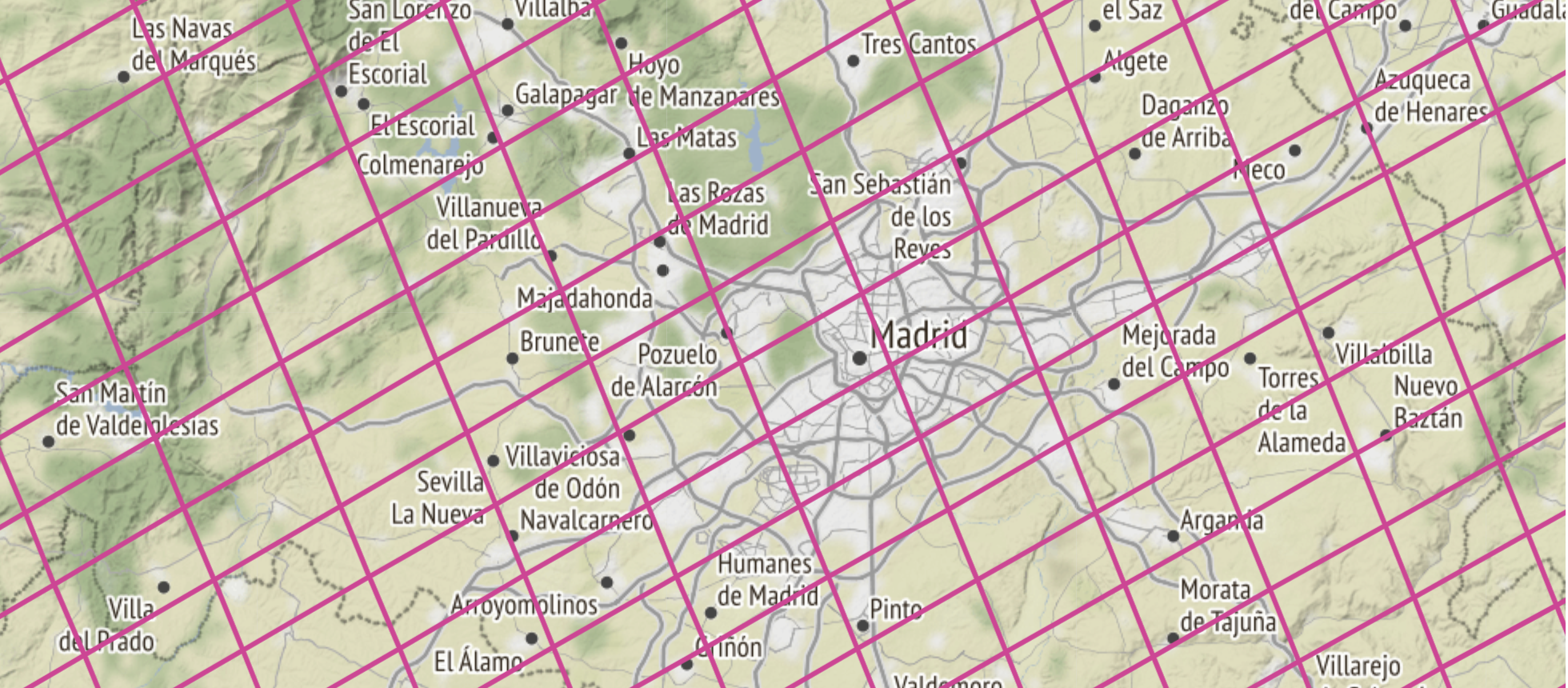
In this use case we are illustrating the satellite data resolution at a city scale, and therefore we are using folium module for plotting. For the folium map the center location is given to Madrid and zoom_start level is set to 10. In the first plot both omi and tropomi pixels are plotted as polygons. The styles (namely color of pixel edges) for each data (omi=plum, tropomi=purple) are defined with style function. The map can be zoomed.
madrid_map = folium.Map(location=[40.416775, -3.703790], zoom_start=8)

style1 = {'fillColor': 'none', 'color': '#dd3497'}
style2 = {'fillColor': 'none', 'color': '#4a1486'}

folium.GeoJson(tropomi, style_function=lambda x:style1).add_to(madrid_map)
folium.GeoJson(omi, style_function=lambda x:style2).add_to(madrid_map)
display(madrid_map)
We can also plot choropleth maps, where each pixel is colored either by the value of pixel area or tropospheric NO2. In this case, since all the needed information (geometry, values) is included in the "omi" and "tropomi" GeoDataFrames, we can use those directly to create a choropleth map. The input that is needed for choropleth includes:
- geo_data: geopandas dataframe, that includes pixel geometry. In this example it is either "omi" or "tropomi"
- data: dataframe of the values we want to show. In this case an additional dataframe is not needed, we will use "omi" or "tropomi"
- columns: column names from the input dataframe that give the keys and value information. Key in this case is variable "pixel_id", and value can be either "NO2" or "area".
First for choropleth map we choose a gray-scaled basemap, and define the colormap for NO2 values. As a colormap we use ColorBrewer palette.
map_omi = folium.Map(location=[40.416775, -3.703790], zoom_start=8, tiles='cartodbpositron')

colormap = branca.colormap.linear.YlGnBu_09.scale(0, 8)
colormap.caption = 'Tropospheric NO2 [Pmol/cm2]'

style_function = lambda x: {"weight": 0.5,
                            'color': ' ',
                            'fillColor': colormap(x['properties']['NO2']),
                            'fillOpacity': 0.6}
folium.GeoJson(
    omi,
    tooltip=folium.GeoJsonTooltip(fields=["pixel_id","NO2"]),
    style_function=style_function
).add_to(map_omi)

# Add the legend to the same canvas
colormap.add_to(map_omi)
display(map_omi)
Similarly, the TROPOMI NO2 values can be plotted on the map, using same styling and colorscale:
map_tropomi = folium.Map(location=[40.416775, -3.703790], zoom_start=8, tiles='cartodbpositron')

folium.GeoJson(
    tropomi,
    tooltip=folium.GeoJsonTooltip(fields=["pixel_id", "NO2"]),
    style_function=style_function
).add_to(map_tropomi)
colormap.add_to(map_tropomi)
display(map_tropomi)